Background

This analysis came about because the dataset was the topic of the Stockholm R User Group (SRUG) Meetup Group Hackathon 2017 (and took me a while to get back to). The task was simply to do something interesting using the dataset.

Text data can be analysed using a variety of different methods: topic modelling, network analysis, sentiment analysis, word frequencies etc. One less commonly applied approach is that of readability, or in other words, linguistic complexity. The thought was that this might reveal an interesting dimension of the data that might be missed by other approaches. It also made for a nice case for demonstrating how readability scores can be applied.

Readability Formulas

Readability formulas were developed as early as the first half of the twentieth century, and therefore used to be calculated by hand. ‘True’ readability is dependent on all sorts of factors: the complexity of the ideas expressed, the logical coherence of the text, the words used etc. What readability formulas measure is usually primarily a function of the most easily quantifiable aspects of readability: words per sentence, syllables per word etc. These quantities are then assembled together in a formula which weights the different components appropriately, to arrive at a readability score. There exist many different readability scores, which differ primarily in the degree of weighting they give to one or the other concept (e.g. sentence length vs word length), or to the way that different components of complexity are assessed (e.g. word length vs membership to an easy word list).

As such, readability formulas tend to be rather crude tools for assessing readability. However, while these measures do not perfectly capture the true readability of a text, they can be especially informative when examining relative changes in large sets of texts to examine changes. For example, I and some friends applied readability formulas to scientific abstracts as a hobby project, finding very strong trend indicating that scientific writing has been growing increasingly complex. Another nice example of their application is in an analysis of US State of the Union addreses, showing them becoming more simple over time.

The idea here was to apply readability fomulas to TED talk transcripts, and to examine whether there have been any changes over time, as well as whether the complexity of the language of the talks had any relation to the popularity of the talks.

The Data Set

The data set is a Kaggle data set available here. The description is as follows:

These datasets contain information about all audio-video recordings of TED Talks uploaded to the official TED.com website until September 21st, 2017. The TED main dataset contains information about all talks including number of views, number of comments, descriptions, speakers and titles. The TED transcripts dataset contains the transcripts for all talks available on TED.com.

Setup

Packages

library(tidyverse)
library(koRpus)
library(stringi)
library(viridis)

The readability package I’ll be using is called koRpus. While it has its quirks, and it tends to be a little bit slower than some equivalent tools in Python, it is quite easy to use and showcases a very comprehensive set of tools. First, we need to install the english language, as below. We install it using the commented code below, and then load it up like a usual library.

# install.koRpus.lang("en")
library(koRpus.lang.en)

Reading in the data

First, I read the transcripts and the information in, join the two, and throw out everything where there was any missing data.

talks <- read_csv('../../data/20190321_ReadabilityTED/ted_main.csv')

Rows: 2550 Columns: 17
── Column specification ────────────────────────────────────────────────────────
Delimiter: ","
chr (10): description, event, main_speaker, name, ratings, related_talks, sp...
dbl  (7): comments, duration, film_date, languages, num_speaker, published_d...

ℹ Use `spec()` to retrieve the full column specification for this data.
ℹ Specify the column types or set `show_col_types = FALSE` to quiet this message.

transcripts <- read_csv('../../data/20190321_ReadabilityTED/transcripts.csv')

Rows: 2467 Columns: 2
── Column specification ────────────────────────────────────────────────────────
Delimiter: ","
chr (2): transcript, url

ℹ Use `spec()` to retrieve the full column specification for this data.
ℹ Specify the column types or set `show_col_types = FALSE` to quiet this message.

alldat <- full_join(talks, transcripts) %>%
  filter(complete.cases(.))

Joining with `by = join_by(url)`

It’s always a good idea to have a bit of a look at your data before running functions that take a long time. I sound like I’m being smart here. I was less smart at the time and had to re-do some steps here and there to my great chagrin. One discovers that there are little surprises hidden in the data, such as these gems:

alldat$transcript[1171]

[1] "(Music)(Applause)(Music)(Applause)(Music)(Applause)(Music)(Applause)"

# Shortened this one a bit for brevity
str_sub(alldat$transcript[1176], start = 2742, 2816)

[1] "\"sh\" in Spanish. (Laughter) And I thought that was worth sharing.(Applause)"

So, there seem to be various audience reactions included in the transcripts wrapped in brackets. Let’s make sure to remove these, as well as save them for later in case they come in handy.

Audience reactions

Here I first removed and saved the bracketed audience actions. I then used stringi to get word counts so that we can remove the cases for which there’s nothing, or not much, left after removing the brackets, for cases like the first example above.

alldat <- alldat %>%
  mutate(bracketedthings = str_extract_all(transcript, pattern = "\\(\\w+\\)"),
         transcript = str_replace_all(transcript, "\\(\\w+\\)", " "),
         word_count = map_dbl(transcript, ~stri_stats_latex(.)[["Words"]]))

Let’s examine these actions a little bit further

actions <- c(unlist(alldat$bracketedthings))
actions <- gsub(pattern = '[\\(\\)]', replacement = '', x = actions)
length(unique(actions))

[1] 202

202 unique actions is a lot… But what are the main ones?

head( sort(table(actions), decreasing = T), 20)

actions
  Laughter   Applause      Music      Video      Audio     Laughs    Singing 
     10224       5429        614        354         56         49         45 
    Cheers Beatboxing   Cheering    English  Whistling          k      Sighs 
        40         24         17         17         17         16         16 
    Guitar      Sings   Audience       Beep   Clapping     Arabic 
        14         13         12         12         10          9

So, most of these actions are too rare to be useful. But the first three could well be helpful for later.

alldat <- alldat %>%
  # Laughter
  mutate(nlolz = stringr::str_count(bracketedthings, '(Laughter)')) %>%
  mutate(lolzpermin = nlolz/(duration/60)) %>%
  
  # Applause
  mutate(napplause = stringr::str_count(bracketedthings, '(Applause)')) %>%
  mutate(applausepermin = napplause/(duration/60)) %>%
  
  # Has Music
  mutate(hasmusic = stringr::str_detect(bracketedthings, '(Music)'))

Warning: There was 1 warning in `mutate()`.
ℹ In argument: `nlolz = stringr::str_count(bracketedthings, "(Laughter)")`.
Caused by warning in `stri_count_regex()`:
! argument is not an atomic vector; coercing

Warning: There was 1 warning in `mutate()`.
ℹ In argument: `napplause = stringr::str_count(bracketedthings, "(Applause)")`.
Caused by warning in `stri_count_regex()`:
! argument is not an atomic vector; coercing

Warning: There was 1 warning in `mutate()`.
ℹ In argument: `hasmusic = stringr::str_detect(bracketedthings, "(Music)")`.
Caused by warning in `stri_detect_regex()`:
! argument is not an atomic vector; coercing

Calculating readability scores

The koRpus package requires that you install TreeTagger first, and set it up accordingly (in its README). This software tokenises the text, as well as classifies words by parts of speech.

So, first we set up a function for treetagging the text. Remember to check the path for your computer.

treetag_text <- function(text) {
  # Write text to temporary file
  temp_file <- tempfile(fileext = ".txt")
  writeLines(text, temp_file)
  
  # Process the file
  treetagged_text <- treetag(temp_file, 
                             lang="en", treetagger="manual", 
                             TT.options=list(path="/home/granville/TreeTagger/", 
                                             preset="en"))
  
  # Clean up temporary file
  unlink(temp_file)
  
  return(treetagged_text)
}

Once this is done, one can just run the koRpus::readability() command on the treetagged text, and you can get all the readability outcomes.

This all takes quite a long time though, so let’s be sure to save the results after each step. And I’ll save after each of the two processes.

# Tagging
alldat_read <- alldat %>%
  filter(word_count > 50) %>%   # Not enough data with <50 words
  mutate(text_tt = map(transcript, ~(treetag_text(.))))

saveRDS(alldat_read, '../../data/20190321_ReadabilityTED/alldat_tagged.rds')

alldat_read <- readRDS('../../data/20190321_ReadabilityTED/alldat_tagged.rds')

# Readability   
alldat_read <- alldat_read %>% 
  mutate(readability = map(text_tt, ~readability(.))) %>% 
  mutate(textstats = map(text_tt, ~koRpus::describe(.))) %>%
  select(-text_tt)

saveRDS(alldat_read, '../../data/20190321_ReadabilityTED/alldat_read.rds')

On the other side of that, we can simply pull out whichever readability score we want to work with. I will use the Flesch-Kincaid age in this analysis. There is both a score, and an age for which that score is considered appropriate, and so I’ll use the latter. This provides a more intuitive way to understand the scores than the raw scores. Though, at the same time, the more easily interpretable scores are also more dangerous: the ease of interpreting them tends to make it easier to make the mistake of forgetting that readability scores are most appropriately interpreted relative to the rest of the texts, rather than as absolute measures of a text’s readability. This is because differences in the particular topic, or the format (e.g. speeches, novels, scientific articles) can result in differences in the estimated age for which the readability is considered to be appropriate. But we’ll just keep this in mind as we press on.

alldat_read <- readRDS('../../data/20190321_ReadabilityTED/alldat_read.rds')

alldat_read <- alldat_read %>% 
  mutate(FKA = map_dbl(readability, c("Flesch.Kincaid", "age")))

Cleaning Again

When we look at the distribution of the readability scores, we can see that not everything looks so dandy.

theme_set(theme_bw())

ggplot(alldat_read, aes(x=FKA)) +
  geom_histogram(fill="grey", colour="black") +
  labs(title="Hmmmm...")

`stat_bin()` using `bins = 30`. Pick better value with `binwidth`.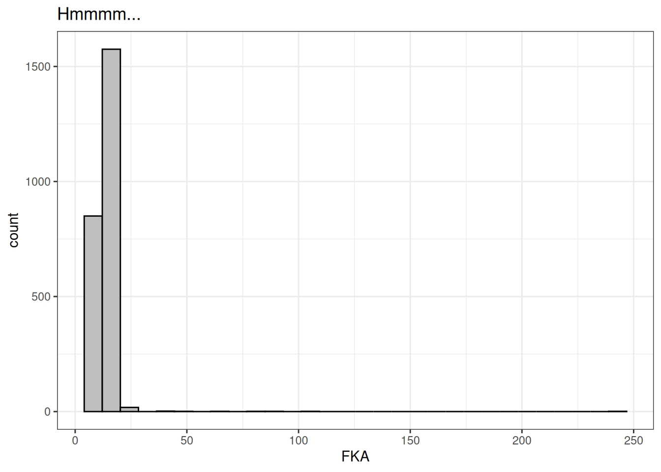

So what are these super complex talks? And what do the most simple talks look like too?

alldat_read <- alldat_read %>% 
  arrange(FKA)

# Most Simple
head(alldat_read$transcript, 1)

[1] "Daffodil Hudson: Hello? Yeah, this is she. What? Oh, yeah, yeah, yeah, yeah, of course I accept. What are the dates again? Pen. Pen. Pen. March 17 through 21. Okay, all right, great. Thanks.Lab Partner: Who was that?DH: It was TED.LP: Who's TED?DH: I've got to prepare.[\"Give Your Talk: A Musical\"]  [\"My Talk\"]♪ Procrastination. ♪ What do you think? Can I help you? Speaker Coach 1: ♪ Let's prepare for main stage. ♪ ♪ It's your time to shine. ♪ ♪ If you want to succeed then ♪ ♪ you must be primed. ♪Speaker Coach 2: ♪ Your slides are bad ♪ ♪ but your idea is good ♪ ♪ so you can bet before we're through, ♪ ♪ speaker, we'll make a TED Talk out of you. ♪Speaker Coach 3: ♪ We know about climate change, ♪ ♪ but what can you say that's new? ♪♪ SC 1: Once you find your focus ♪ ♪ then the talk comes into view. ♪SC 2: ♪ Don't ever try to sell something ♪ ♪ from up on that stage ♪ ♪ or we won't post your talk online. ♪All: ♪ Somehow we'll make a TED Talk out of you. ♪ SC 1: Ready to practice one more time?DH: Right now?Stagehand: Break a leg.DH: ♪ I'll never remember all this. ♪ ♪ Will the clicker work when I press it? ♪ ♪ Why must Al Gore go right before me? ♪ ♪ Oh man, I'm scared to death. ♪ ♪ I hope I don't pass out onstage ♪ ♪ and now I really wish I wasn't wearing green. ♪All: ♪ Give your talk. ♪SC 1: ♪ You must be be sweet like Brené Brown. ♪All: ♪ Give your talk. ♪SC 2: ♪ You must be funny like Ken Robinson. ♪All: ♪ Give your talk. ♪SC 3: ♪ You must be cool like Reggie Watts ♪All: ♪ and bring out a prop like Jill Bolte Taylor. ♪DH: ♪ My time is running over. The clock now says nil. ♪ ♪ I'm saying my words faster. Understand me still. ♪ ♪ I'm too nervous to give this TED Talk. ♪All: ♪ Don't give up. Rehearse. You're good. ♪ ♪ We'll edit out the mistakes that you make. ♪ ♪ Give your talk. ♪DH: ♪ I will be big like Amy Cuddy. ♪All: ♪ Give your talk. ♪DH: ♪ I will inspire like Liz Gilbert. ♪All: ♪ Give your talk. ♪DH: ♪ I will engage like Hans Rosling ♪ ♪ and release mosquitos ♪ ♪ like Bill Gates. ♪SC 2: ♪ I'll make a TED Talk out of you. ♪ ♪ I'll make a TED Talk out of you. ♪ ♪ I'll make a TED Talk out of you. ♪ ♪ I'll make a TED Talk out of you. ♪ ♪ I'll make a TED Talk out of you. ♪ [\"Brought to you by TED staff and friends\"] "

# Most Complex
tail(alldat_read$transcript, 1)

[1] "The first time I uttered a prayer was in a glass-stained cathedral.I was kneeling long after the congregation was on its feet,dip both hands into holy water,trace the trinity across my chest,my tiny body drooping  like a question markall over the wooden pew.I asked Jesus to fix me,and when he did not answerI befriended silence in the hopes that my sin would burnand salve my mouth would dissolve like sugar on tongue,but shame lingered as an aftertaste.And in an attempt to reintroduce me to sanctity,my mother told me of the miracle I was,said I could grow up  to be anything I want.I decided to be a boy.It was cute.I had snapback, toothless grin,used skinned knees as street cred,played hide and seek with  what was left of my goal.I was it.The winner to a game  the other kids couldn't play,I was the mystery of an anatomy,a question asked but not answered,tightroping between awkward boy and apologetic girl,and when I turned 12, the boy phase wasn't deemed cute anymore.It was met with nostalgic aunts who missed seeing my knees in the shadow of skirts,who reminded me that my kind of attitude would never bring a husband home,that I exist for heterosexual marriage and child-bearing.And I swallowed their insults along with their slurs.Naturally, I did not come out of the closet.The kids at my school opened it without my permission.Called me by a name I did not recognize,said \"lesbian,\"but I was more boy than girl, more Ken than Barbie.It had nothing to do with hating my body,I just love it enough to let it go,I treat it like a house,and when your house is falling apart,you do not evacuate,you make it comfortable enough to house all your insides,you make it pretty enough to invite guests over,you make the floorboards strong enough to stand on.My mother fears I have named myself after fading things.As she counts the echoes left behind by Mya Hall, Leelah Alcorn, Blake Brockington.She fears that I'll die without a whisper,that I'll turn into \"what a shame\" conversations at the bus stop.She claims I have turned myself into a mausoleum,that I am a walking casket,news headlines have turned my identity into a spectacle,Bruce Jenner on everyone's lips while the brutality of living in this bodybecomes an asterisk  at the bottom of equality pages.No one ever thinks of us as humanbecause we are more ghost than flesh,because people fear that my gender expression is a trick,that it exists to be perverse,that it ensnares them without their consent,that my body is a feast for their eyes and handsand once they have fed off my queer,they'll regurgitate all the parts they did not like.They'll put me back into the closet, hang me with all the other skeletons.I will be the best attraction.Can you see how easy it is to talk people into coffins,to misspell their names on gravestones.And people still wonder why there are boys rotting,they go away in high school hallwaysthey are afraid of becoming another hashtag in a secondafraid of classroom discussions becoming like judgment dayand now oncoming traffic is embracing more transgender children than parents.I wonder how long it will bebefore the trans suicide notes start to feel redundant,before we realize that our bodies become lessons about sinway before we learn how to love them.Like God didn't save all this breath and mercy,like my blood is not the wine that washed over Jesus' feet.My prayers are now getting stuck in my throat.Maybe I am finally fixed,maybe I just don't care,maybe God finally listened to my prayers.Thank you.  "

They’re both songs! This is something that will trip up readability scores: they’re made for full sentences. Songs don’t have the usual sentences, and, at least in the second case, they are considered as one long sentence. Let’s take a look.

alldat_read <- alldat_read %>%
  mutate(sentences = map_dbl(textstats, 'sentences'),
         sentencelength = map_dbl(textstats, 'avg.sentc.length'))
 
ggplot(alldat_read, aes(x=sentencelength)) +
  geom_histogram(fill="grey", colour="black") +
  labs(title="Average Sentence Lengths")

`stat_bin()` using `bins = 30`. Pick better value with `binwidth`.

Warning: Removed 2 rows containing non-finite outside the scale range
(`stat_bin()`).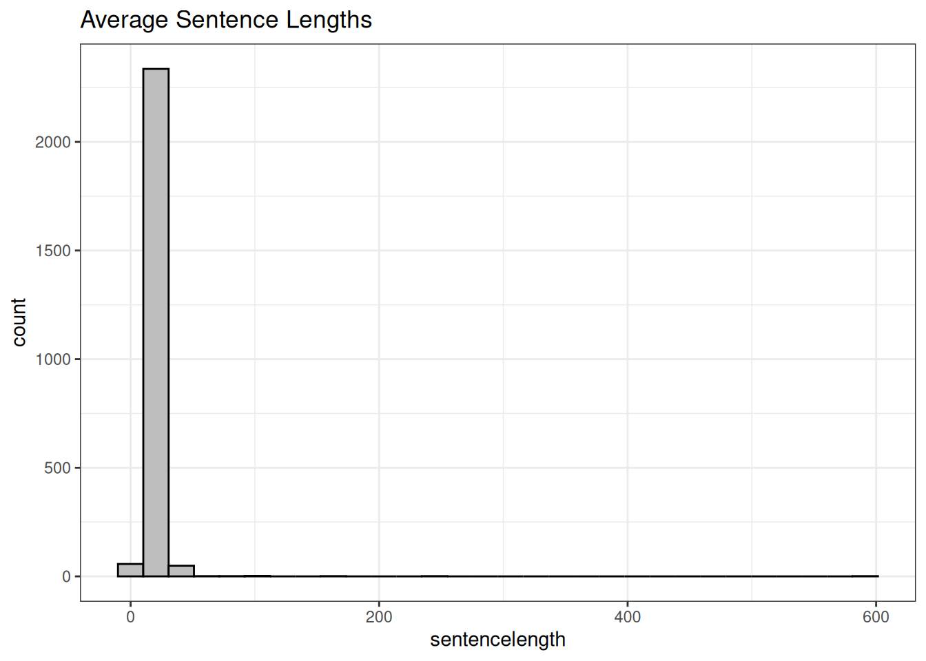

So let’s try to remove the bad cases to the right, choosing a limit of average 40 words per sentence, as well removing those talks including music using the variable we created earlier from the audience reactions, and see how everything looks again

readdat <- alldat_read %>%
  select(-bracketedthings) %>%
  filter(sentencelength < 40,
         hasmusic==FALSE)

ggplot(readdat, aes(x=FKA)) +
  geom_histogram(fill="grey", colour="black") +
  labs(title="Muuuuch better!")

`stat_bin()` using `bins = 30`. Pick better value with `binwidth`.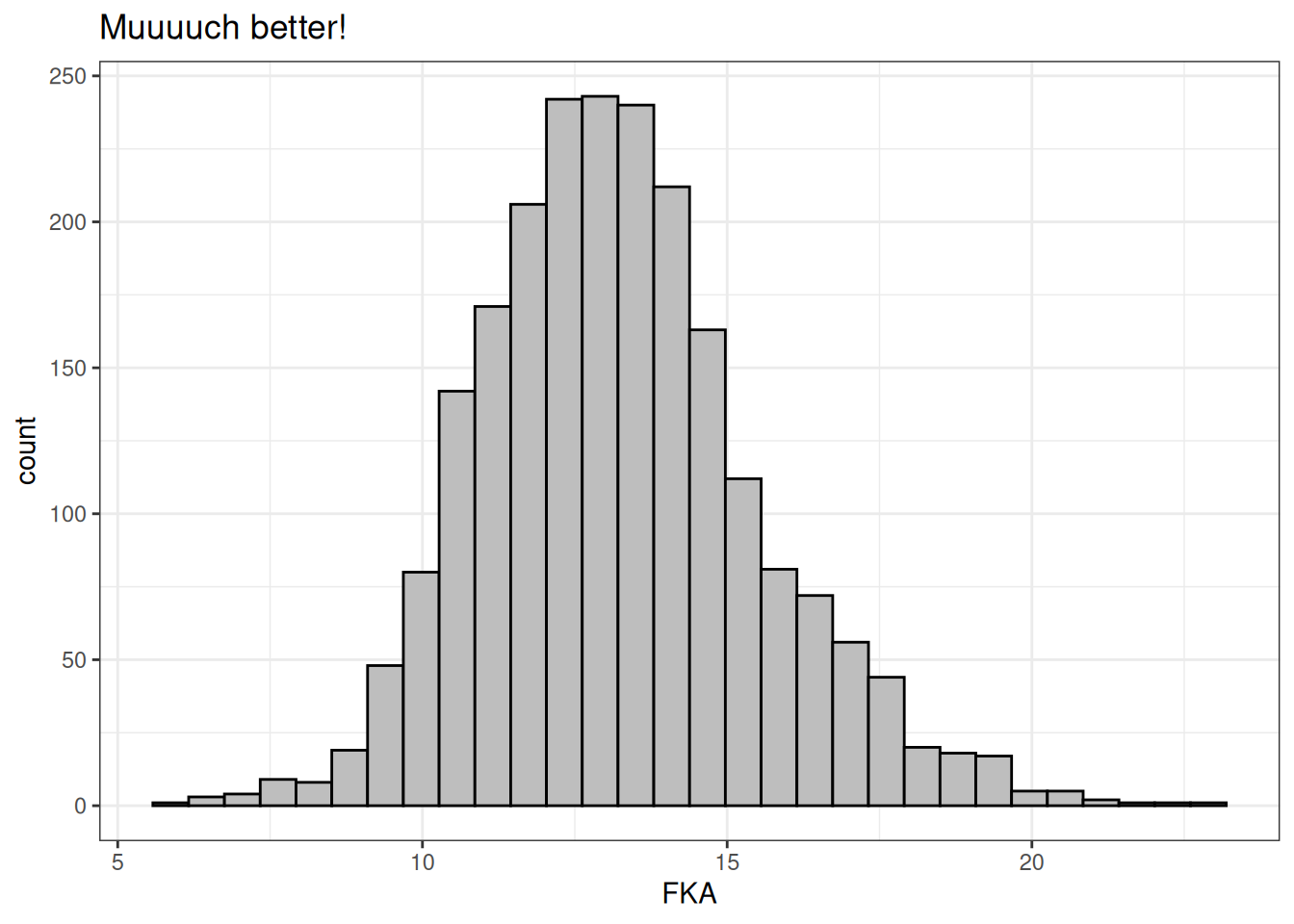

Now that’s a normal distribution if ever I saw one! This data looks pretty ripe for digging into now!

Exploration

In order to look at trends over time, let’s first fix up the dates. The dates are UNIX timestamps, so I’ll first convert these to more normal dates.

readdat <- readdat %>% 
  mutate(published_date = as.POSIXct(published_date, origin="1970-01-01"),
         published_date = as.Date(published_date))

Views per day

As a crude indicator of interest in each video, I’ll calculate the number of views per day elapsed since the video was published, in order not to be biased by the time that the video has been available in which to be viewed. The dataset describes videos on the TED.com website published before September 21st 2017, with the dataset created on September 25th according to one of the comments on the page.

readdat <- readdat %>% 
  mutate(days = as.Date("2017-09-25") - published_date,
         days = as.numeric(days),
         viewsperday = views/days)

ggplot(readdat, aes(x=viewsperday)) +
  geom_histogram(fill="grey", colour="black")

`stat_bin()` using `bins = 30`. Pick better value with `binwidth`.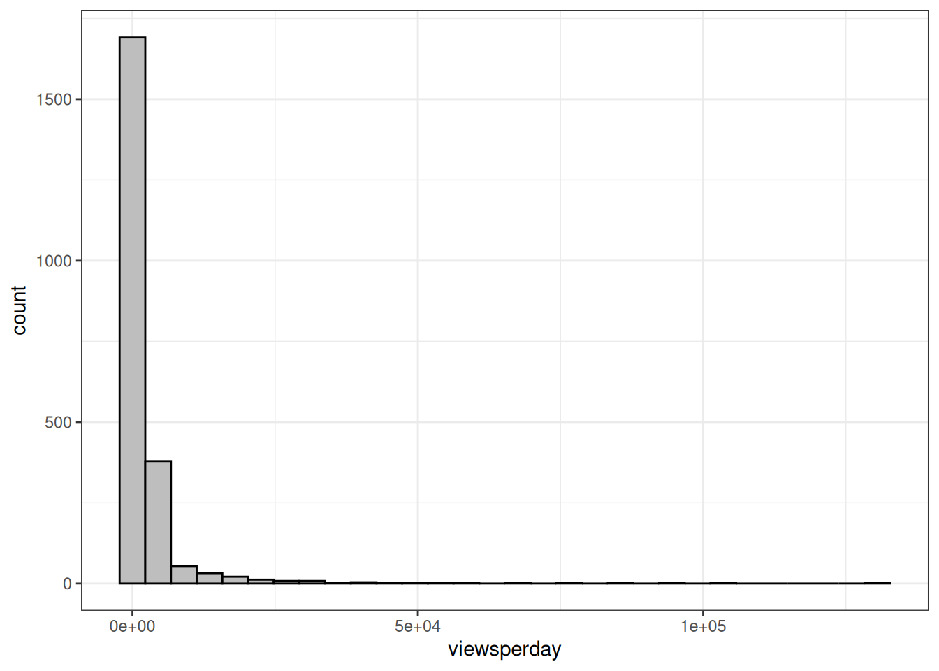

Looks like this might be more useful with a log transformation

readdat <- readdat %>% 
  mutate(log_vpd = log10(viewsperday))

ggplot(readdat, aes(x=log_vpd)) +
  geom_histogram(fill="grey", colour="black")

`stat_bin()` using `bins = 30`. Pick better value with `binwidth`.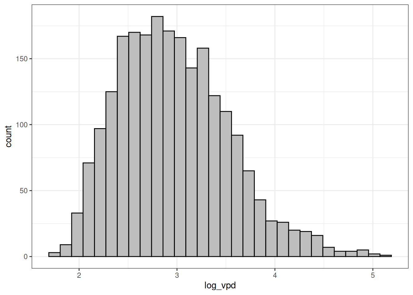

That looks much better! Let’s take a look at the trend over time.

ggplot(readdat, aes(x=published_date, y=log_vpd)) +
  geom_point() +
  labs(y="Log views per day")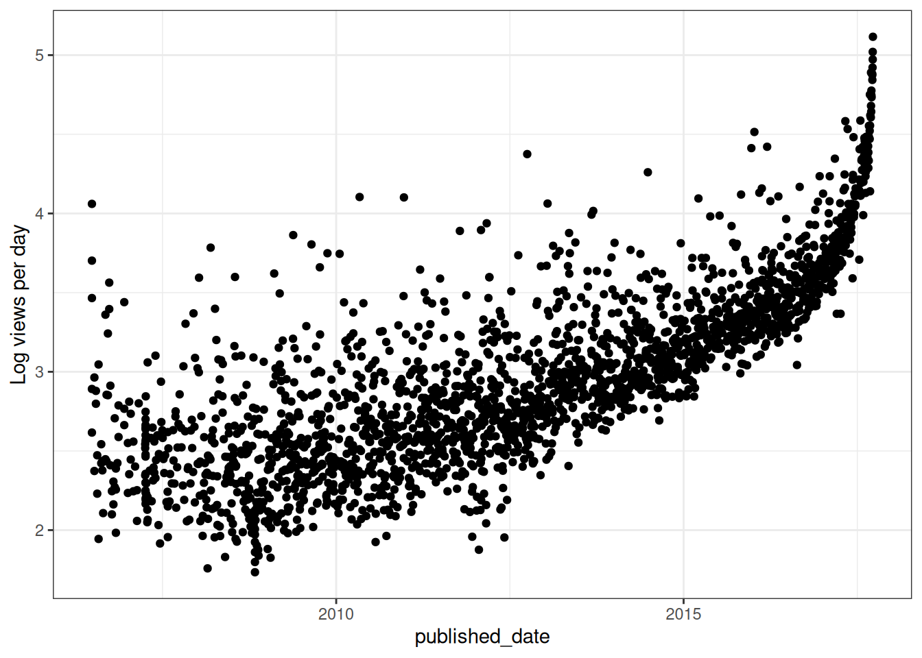

I suspect that the date that the data was frozen is probably wrong. Or something else is funny here. Maybe we can just use the raw views data instead, but I would then remove those datapoints in the last few months which haven’t been around long enough to go viral.

readdat$too_recent <- readdat$published_date > as.Date("2017-04-01")

ggplot(readdat, aes(x=published_date, y=log10(views))) +
  geom_point(aes(colour=too_recent))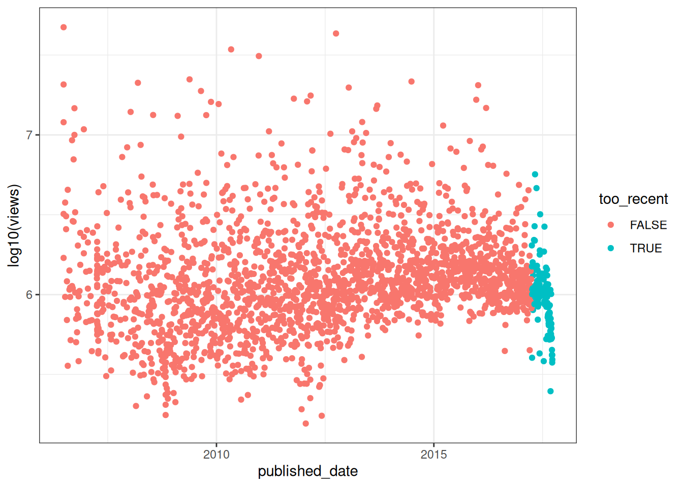

That looks ok. And they actually also look to be affected by published date to a surprisingly small extent. Therefore I think it makes sense to just use the views figures, and to cut out the most recent talks to avoid their bias.

readdat <- readdat %>% 
  filter(published_date < as.Date("2017-04-01"))

Changes over Time

As a first step, let’s take a look at whether there are any trend in readability over time.

corstrength <- cor(readdat$FKA, as.numeric(readdat$published_date))

readability_trend <- ggplot(readdat, aes(x=published_date, y=FKA)) +
  geom_point(aes(colour=log10(views))) +
  scale_colour_viridis(option = 'D', 'Log(Views)') +
  geom_smooth(colour="red") +
  geom_smooth(method="lm") +
  labs(title='Readability over Time',
       subtitle=paste0("Linguistic complexity has increased over time: R = ",round(corstrength, 2)),
       y='Flesch-Kincaid Readability (Age)', x='Published Date')

readability_trend

`geom_smooth()` using method = 'gam' and formula = 'y ~ s(x, bs = "cs")'
`geom_smooth()` using formula = 'y ~ x'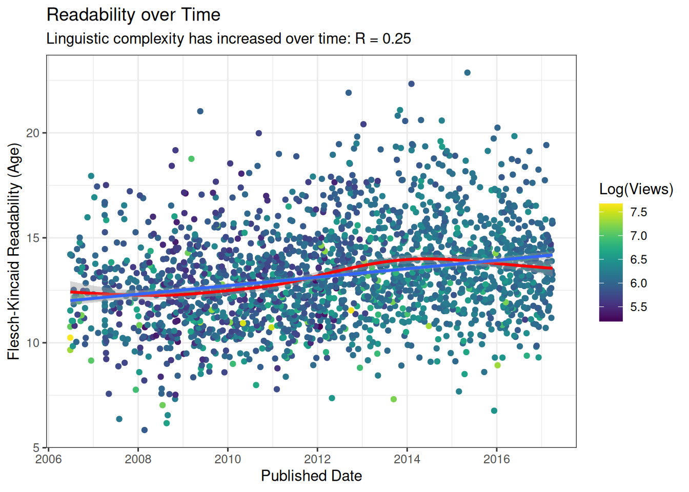

This is actually rather stronger than I anticipated, and seems to be a pretty clear result of talks becoming more complex over time. The linear trend is the same as we saw in the scientific literature. Interestingly, from the smooth model fit to the data, there appears to have been a peak in complexity around the beginning of 2014, which has perhaps tapered off, but I wouldn’t be able to begin to start to speculate about what might have caused that, so it could well be nothing.

Viewership

Let’s also take a look then at how readability relates to views.

readability_popularity <- ggplot(readdat, aes(x=FKA, y=log10(views))) +
  geom_point() +
  labs(title='Readability Score and Views',
       subtitle="No strong relation, but notice the gap top right",
       x='Flesch-Kincaid Readability (Age)',
       y='Log(Views)')

readability_popularity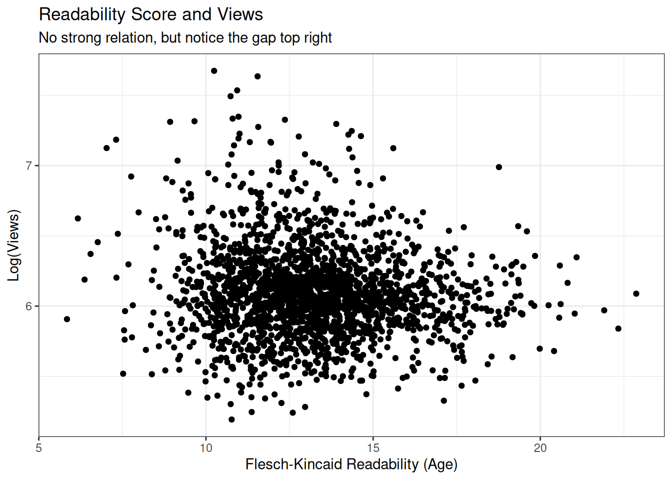

We can see here that there are many talks which are highly readable (left) and with many views, however very few which are complex and also popular. Let’s take a closer look at this.

For this, I will divide the readability scores into deciles, and compare the distributions of the views.

readdat <- readdat %>%
  mutate(read_percentile = cut(FKA, 10),
         read_percentile_num = as.numeric(read_percentile)*10,
         read_percentile_num_mid = read_percentile_num-5) %>%
  group_by(read_percentile_num) %>%
  mutate(meanRead = mean(FKA)) %>%
  ungroup()

readability_quantile <- ggplot(readdat, aes(x=read_percentile_num_mid,
                                            y=log10(views), fill=meanRead,
                                            group=read_percentile_num)) +
  geom_boxplot() +
  scale_fill_viridis('Mean \nReadability \nAge', direction = -1) +
  labs(title='Readability Percentile and Views',
       subtitle="Especially simple talks are most popular, \nand especially complex talks have uniformly few views",
       x='Readability Percentile (Simplest to Hardest)',
       y='Views (Log10)')

readability_quantile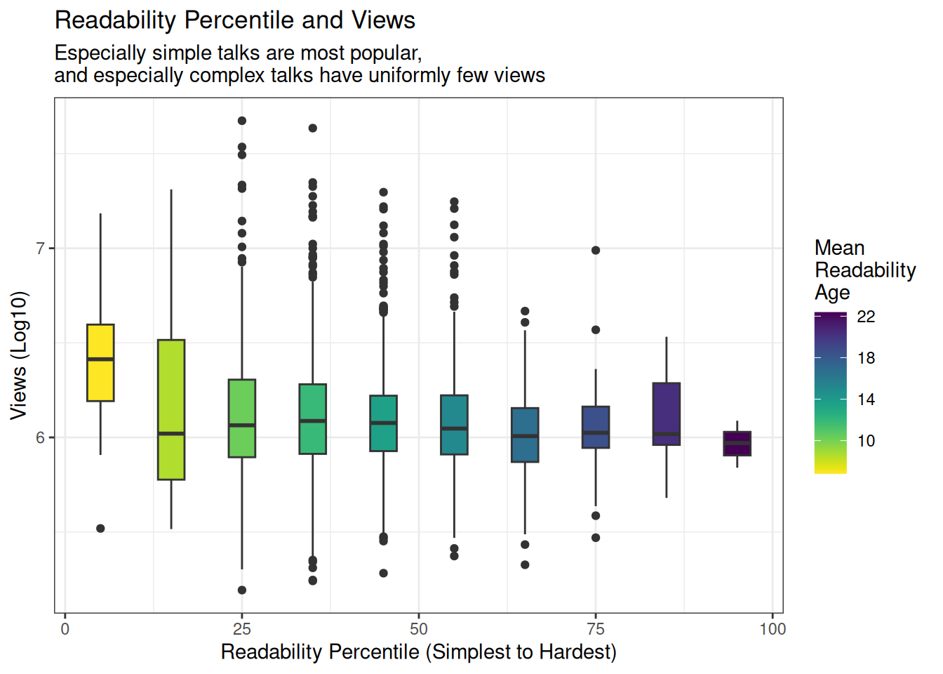

Topics

It would have been nice to separate the data into different topics or sections, but unfortunately that data isn’t quite so clear. What we do have is a set of tags. Let’s maybe take a little look at that data and see whether we might be able to try to see which topics are most complex and which are most simple.

readdat$tags[[1]]

[1] "['collaboration', 'entertainment', 'humor', 'physics']"

topicdat <- readdat %>%
  mutate(tags = str_match_all(tags, pattern = "\\'(\\w+)\\'"),
         tags = map(tags, ~.x[,2]))

Let’s examine these actions a little bit further

tags <- c(unlist(topicdat$tags))
length(unique(tags))

[1] 328

That looks like too many - this data will be too sparse. But let’s see what the most common are.

head( sort(table(tags), decreasing = T), 30)

tags
   technology       science       culture          TEDx        design 
          612           500           430           358           350 
     business        health    innovation entertainment       society 
          309           202           191           186           165 
       future           art       biology communication     economics 
          163           160           160           158           147 
        brain      medicine   environment collaboration    creativity 
          142           142           140           138           135 
     humanity      activism     education     invention     community 
          134           132           132           125           121 
      history      children      politics    psychology         women 
          120           112           109           108           108

These all have reasonable numbers of talks. Let’s compare them. Keep in mind that the same talks might belong to multiple categories, so there will be overlap.

topics <- names(head( sort(table(tags), decreasing = T), 30))

topic_read <- topicdat %>% 
  select(FKA, tags, views)

selectbytopic <- function(topic, data) {
  filter(data, map_lgl(tags, ~topic %in% .x))
}

topic_readgroups <- map(topics, ~selectbytopic(.x, topic_read))
names(topic_readgroups) <- topics

topic_readgroups <- bind_rows(topic_readgroups, .id="Tag") %>% 
  select(-tags) %>% 
  group_by(Tag) %>% 
  mutate(meanRead = mean(FKA),
         meanViews = mean(views)) %>% 
  ungroup()

So let’s take a look at the readability of the different topics. Let’s first look by views

views_topics <- topic_readgroups %>% 
  arrange(-meanViews) %>% 
  mutate(Tag = fct_inorder(Tag)) %>% 
  ggplot(aes(x=Tag, y=log10(views), fill=meanRead, group=Tag)) +
  geom_boxplot() +
  scale_fill_viridis('Mean \nReadability \nAge', direction = -1) +
  labs(title='Views by Tags',
       subtitle="Psychology and brain talks get more views, but the tags don't differ greatly otherwise",
       x='Tag',
       y='Views (Log10)') +
  theme(axis.text.x = element_text(angle = 60, hjust = 1))

views_topics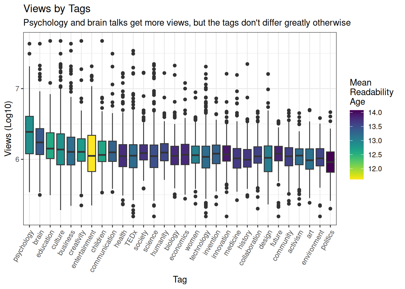

Interesting to see such a strong preference for psychology and brain talks. We can also already see that the entertainment tag appears to be associated with more readable transcripts. But let’s take a look at the distributions.

readability_topics <- topic_readgroups %>% 
  arrange(-meanRead) %>% 
  mutate(Tag = fct_inorder(Tag)) %>% 
  ggplot(aes(x=Tag, y=FKA, fill=log10(meanViews), group=Tag)) +
  geom_boxplot() +
  scale_fill_viridis('Mean \nViews \n(Log10)') +
  labs(title='Readability by Tags',
       subtitle="Politics are complex, entertainment is simple, but the others don't differ much",
       x='Tag',
       y='Flesch-Kincaid Readability Age') +
  theme(axis.text.x = element_text(angle = 60, hjust = 1))

readability_topics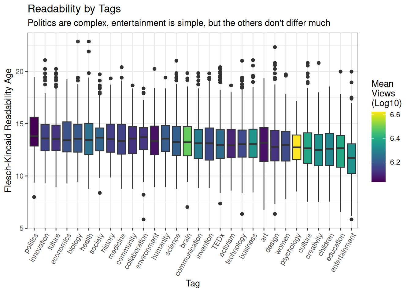

That politics and economics should be most complex, and that education, children and entertainment should be simplest, makes intuitive sense. It definitely seems like, despite being quite crude instruments, that the readability formulas do a pretty good job of capturing the real differences in complexity.

Also, interesting to note above that the topics of the talks don’t appear to be completely driving the differences in readability: brain talks are very popular, but reasonably complicated; while entertainment talks are very simple, but not massively popular.

Audience Laughter

Next, let’s take a look at how funny talks were compared to their complexity. We saved the laughs per minute earlier, so we can use that data. Let’s filter for the laughs for which laughter was recorded first though.

lolpermin <- readdat %>%
  filter(lolzpermin > 0) %>%
  ggplot(aes(x=FKA, y=log10(lolzpermin), colour=log10(views))) +
    geom_point() +
    geom_smooth(method="lm") +
    labs(title='Readability and Laughs',
         subtitle='Simpler talks get more laughs',
         x='Flesch-Kincaid Readability (Age)',
         y='Lolz/minute (Log10)') +
  scale_colour_viridis(option = 'D', 'Log(Views)')

lolpermin

`geom_smooth()` using formula = 'y ~ x'

Warning: The following aesthetics were dropped during statistical transformation:
colour.
ℹ This can happen when ggplot fails to infer the correct grouping structure in
  the data.
ℹ Did you forget to specify a `group` aesthetic or to convert a numerical
  variable into a factor?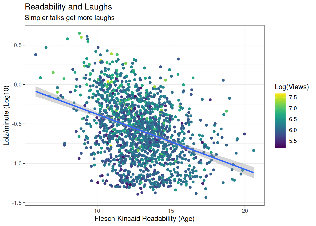

Engagement

And engagement. Let’s make a crude marker of engagement by taking the log of the number of ratings per view. First, we need to extract the number of ratings, and then we can calculate engagement.

readdat$ratings[[1]]

[1] "[{'id': 23, 'name': 'Jaw-dropping', 'count': 402}, {'id': 7, 'name': 'Funny', 'count': 1637}, {'id': 1, 'name': 'Beautiful', 'count': 59}, {'id': 22, 'name': 'Fascinating', 'count': 267}, {'id': 9, 'name': 'Ingenious', 'count': 116}, {'id': 21, 'name': 'Unconvincing', 'count': 15}, {'id': 10, 'name': 'Inspiring', 'count': 57}, {'id': 25, 'name': 'OK', 'count': 126}, {'id': 3, 'name': 'Courageous', 'count': 72}, {'id': 24, 'name': 'Persuasive', 'count': 14}, {'id': 26, 'name': 'Obnoxious', 'count': 52}, {'id': 11, 'name': 'Longwinded', 'count': 56}, {'id': 8, 'name': 'Informative', 'count': 9}, {'id': 2, 'name': 'Confusing', 'count': 6}]"

get_ratingcount <- function(ratingtext) {
  ratingcount <- stringr::str_match_all(ratingtext, "'count': (\\d*)")[[1]][,2]
  sum(as.numeric(ratingcount))
}

readdat <- readdat %>% 
  mutate(ratingcount = map_dbl(ratings, ~get_ratingcount(.x)),
    engagement = log10(ratingcount/views))

Right, now let’s see how it looks

engagement <- readdat %>%
  ggplot(aes(x=FKA, y=engagement, colour=log10(views))) +
    geom_point() +
    geom_smooth(method="lm") +
  scale_colour_viridis('Log Views') +
    labs(title='Readability and Engagement',
         subtitle='Simpler talks get more engagement',
         x='Flesch-Kincaid Readability (Age)',
         y='Engagement (Log (Ratings / Views)')

engagement

`geom_smooth()` using formula = 'y ~ x'

Warning: The following aesthetics were dropped during statistical transformation:
colour.
ℹ This can happen when ggplot fails to infer the correct grouping structure in
  the data.
ℹ Did you forget to specify a `group` aesthetic or to convert a numerical
  variable into a factor?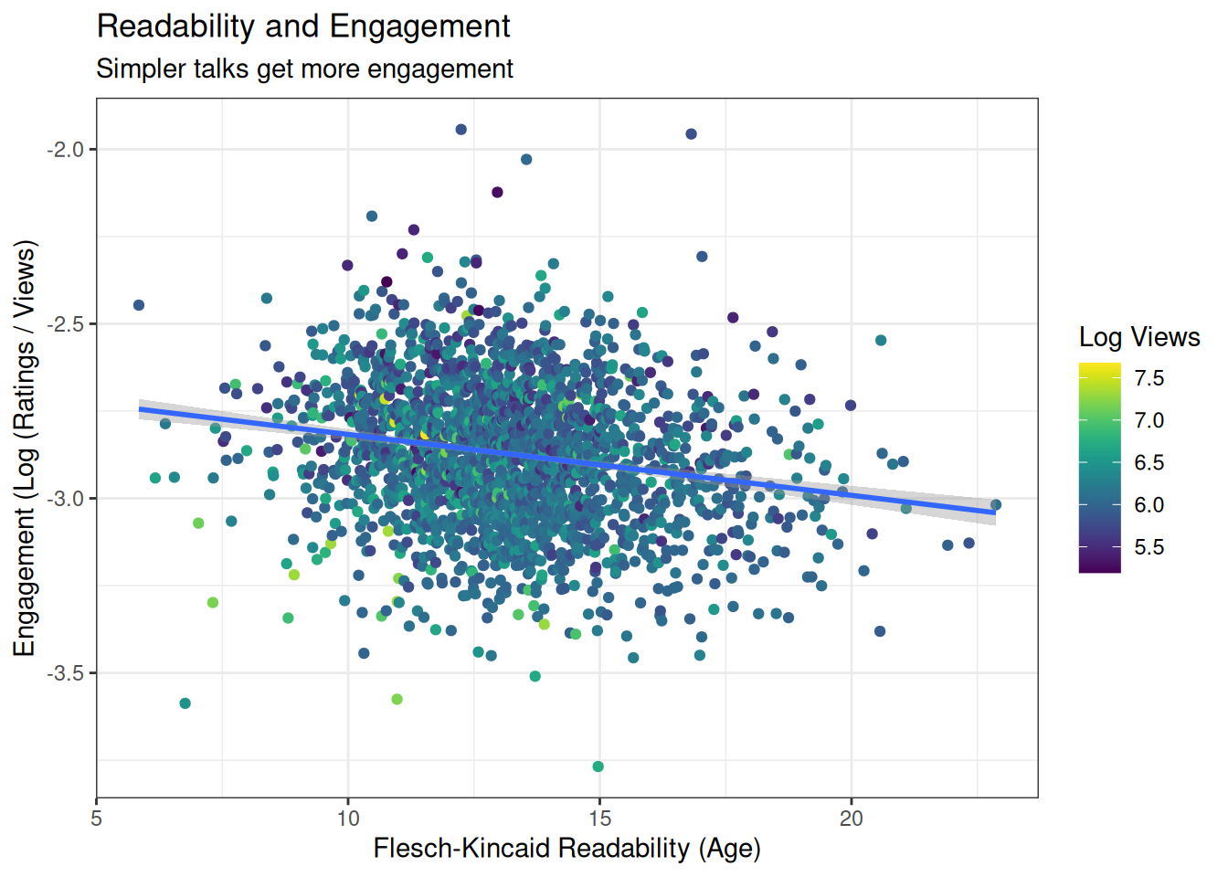

Conclusions

In this analysis, and much to my surprise I must admit, we found that linguistic complexity, measured using readability formulas, appears to be related to pretty much everything we looked at. It seemed to be changing over time, with talks growing more complex. We showed that talks with high complexity had universally low viewership, and that simpler talks are not only more viewed, but also get more laughs, and get more engagement. We further showed that politics and economics talks tend to be more complicated, while talks about education, children and entertainment tend to be more simple.

And, lastly, if you should ever be preparing to do a TED talk: keep it simple!